Graphs #3
This week I implemented circle layout and two different subtypes of it.
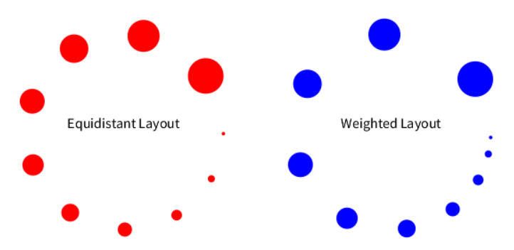
The distinction between them is in how they treat the gap between vertices in comparison to their size.
Equidistant makes sure that the gap is the same, no matter which size is the vertex. Weighted circle expands the gap, as the size of a vertex is getting bigger.
To continue with learning about graphs, we need to understand DFS of depth first search.
DFS - depth first search
In BFS, we were taking one node and looking first for all his neighbours, so from a perspective of that node, our view is breadth first oriented. Following this logic, DFS will have a depth first oriented view from a chosen node. Simply said, we will choose one neighbour and take him, choose one of his neighbours and so on.
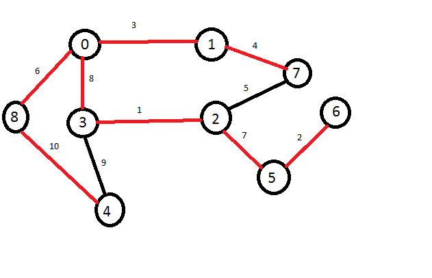
Let’s work through the same example we used last week.
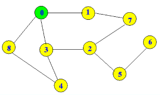
Again, we start from vertex 0 and visit his first neighbour. Have in mind, that we can only choose vertices, that haven't been visited before. So when we find ourself in a dead end (no unvisited neighbours, but we haven't finished the algorithm), we take a step back, take previously visited vertex, and look for another neighbour of his.
Strategy for choosing vertex is the smallest number.
Our process will go like this:
0 -> 1, 1 -> 7, 7 -> 2, 2 -> 3, 3 -> 4, 4 -> 8
8 -> At this moment we have no unvisited neighbours, so we take a step back.
4 -> At this moment we have no unvisited neighbours, so we take a step back.
3 -> At this moment we have no unvisited neighbours, so we take a step back.
2 -> 5, 5 -> 6, 6 has no neighbours, so we take a step back.
5 -> At this moment we have no unvisited neighbours, so we take a step back.
2 -> At this moment we have no unvisited neighbours, so we take a step back.
7 -> At this moment we have no unvisited neighbours, so we take a step back.
1 -> At this moment we have no unvisited neighbours, so we take a step back.
0 -> At this moment we have no unvisited neighbours, we there are no more steps back to take.
With this out DFS algorithm is finished.
There are many uses for this algorithm, like partitioning the vertices into connected components, checking if a graph is bipartite, finding a circle, topological sort, etc.
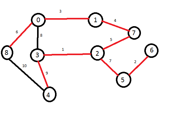
These two algorithms are basic ones, starting from here, we have: Kosaraju's algorithm for computing strongly connected components in a Digraph (there is a reachability in both directions); Prim's algorithm, Kruskal's algorithm, both used for finding the minimal spanning tree of a graph (acyclic, connected subgraph, that contains all vertices and has a minimal weighted sum); Dijkstra's algorithm for finding shortest path in a weighted directed graph and many others.
Prim’s algorithm:
Dijkstra’s algorithm: